Tangram II first steps

Tangram II is a very flexible tool to construct, solve and simulate stochastic models.  It comes with a manual, and the objective of this page is to give you a first contact with the tool before (or in parallel as) you read the manual. Always remember: READ THE MANUAL! :-)


Requirements

  1. A GNU/Linux distribution:
    Tangram-II is developed on Mandrake Linux, but it should run in any current GNU/Linux distribution. We already tested it in Conectiva, Slackware and Debian.
  2. GNU/Linux tools:
    Development tools such as gcc, make, bison, flex and Java Development Kit are needed to compile and run Tangram-II. You also need to install gnuplot to be able to plot graphs from the Tangram-II interface.
    You can get Java Software Development Kit (SDK) from: http://java.sun.com
  3. Tgif:
    Tgif, with version > 4.1.43.93, is needed to create a model and to run interactive simulations in Tangram-II.
    You can get tgif from here
  4. Tangram-II source code
    You can download Tangram-II source code from http://www.land.ufrj.br

Compiling Tangram-II

First of all, you need to check the requirements listed above. Then, download the file tangram2-3.0.tar.gz, and run:

    tar xvfz tangram2-3.0.tar.gz
    cd tangram2-3.0
    ./configure
    make
    make install      

Usage

In this section we will assume that Tangram-II is installed in /usr/local/Tangram2.

  1. Copy the directory /usr/local/Tangram2/examples to your home directory so that you may modify the examples, working with them without destroying the original files.

    Type: cp /usr/local/Tangram2/examples ~/ -R

  2. Run tangram2.

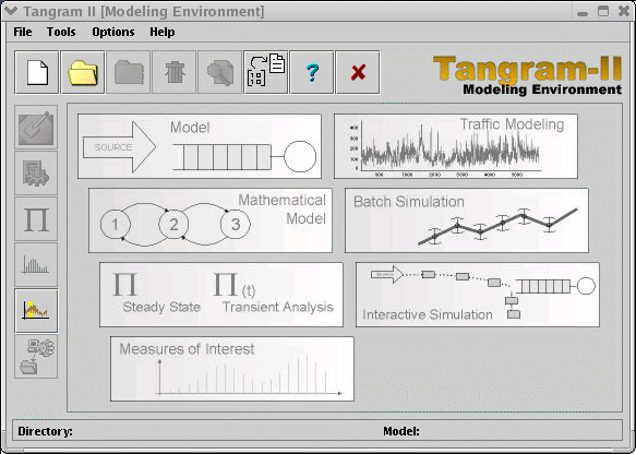
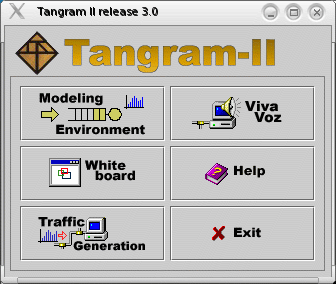
  3. You will get the following screen :
Main Window

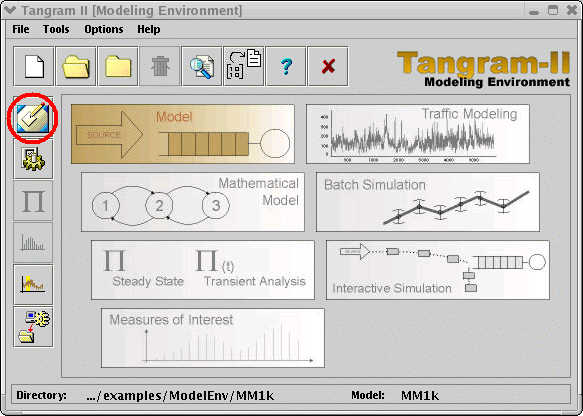
  1. Click on the "Modeling Environment" button.  You will get the "Modeling Environment":

Model Environment

  1. Click on File, Open, and select the file  ~/examples/ModelEnv/MM1k/MM1k.obj.  We will work with the M/M/1/k model.  The source rate is lambda=10 packets per unit of time, and the server service rate is mu=20 packets per unit of time. The maximum queue size is k=10.  In the manual there is a tutorial about how to construct this model.  Here we will just modify an example which was previously created.

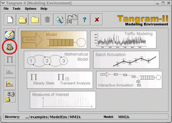
  1. Now open the model description. Click on the "Model Specification" button, as pointed out in the figure below.

    modelenv


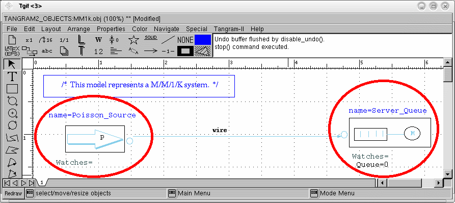
  1. A TGIF screen will be displayed. TGIF (Tangram Graphic Interface Facility) is a 2d drawing program developed for Tangram-II.
tgif2

  1. In the left, you see a Poisson source.  In the right, a Poisson server (with a queue).  You may double click in the objects marked with a red circle in order to see their descriptions.

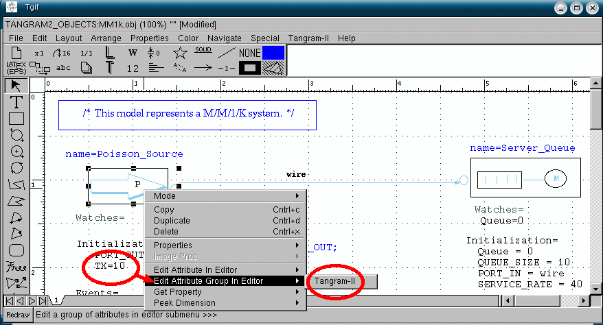
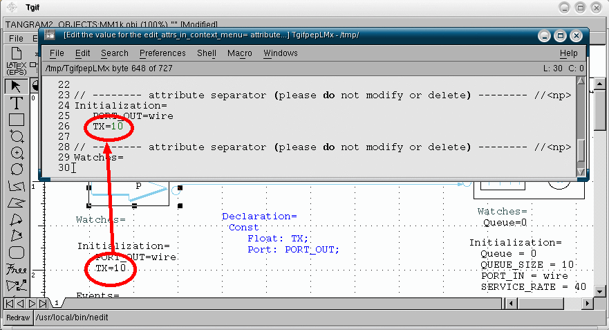
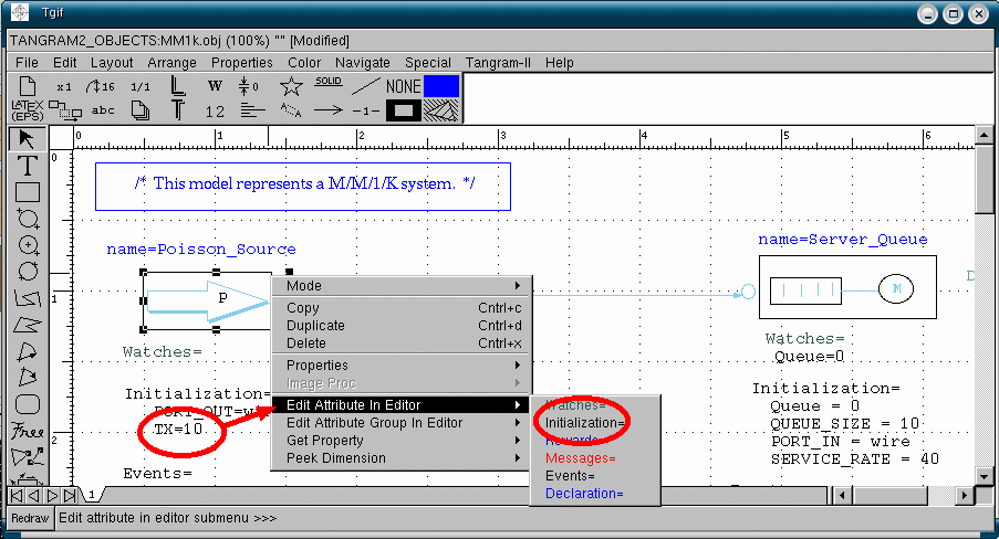
  1. In order to make changes in the model you may right click on the object which you want to alter, and select "Edit attribute in group editor/Tangram-II". Then use your preferred text editor (the default is vi) to modify your model attribute - for instance, the Poisson source rate (from 10 to 15, in the "Intialization" attribute, as shown in the picture below).

  2. editattrib.gif

    editattrib.gif


    excl


    Pay attention! Always remember to save the text file which your are editing with your preferred text editor after you make the desired modifications, before proceding to the next step!


    excl


    You may change the preferred text editor including one of the following lines to your ~/.Xdefaults file:
    Tgif*Editor: nedit -svrname '%s' '%s' Tgif*Editor: xterm -title '%s' -e vi '%s' Tgif*Editor: kwrite -title<br><br> '%s' '%s' Also, check if you have the followings lines in your ~/.Xdefaults file:
    Tgif.MaxAttributeGroups: 1 Tgif.AttributeGroup0:Tangram-II:Events:Messages:Declaration:Rewards:Initialization:Watches
    Then, run

    xrdb ~/.Xdefaults

    One more note: if you want syntax highlight with NEdit, you may copy this file to your home directory, saving it as ~/.nedit.

    Also, if you experience problems when trying to instantiate an object, you may try to get the following version of Xdefaults, edit the paths to the files referenced properly, and copy it to your home directory (save it as ~/.Xdefaults). Then, type

    xrdb ~/.Xdefaults

    excl
    Deprecated: In order to make changes in the model you may also right click on the object which you want to alter, and select "Edit attribute in editor". Then, use your preferred text editor (the default is vi), to modify your model attribute. To modify the Poisson source rate from 10 to 15, in the "Intialization" attribute, see the figure below.  


editattrib.gif


  1. Ok. Now save the file (in TGIF, click on "file", "save").  And go back to the "Modeling Environment".


excl


Pay attention! Always remember to save the TGIF file after you make the desired modifications, before proceding to the next step!


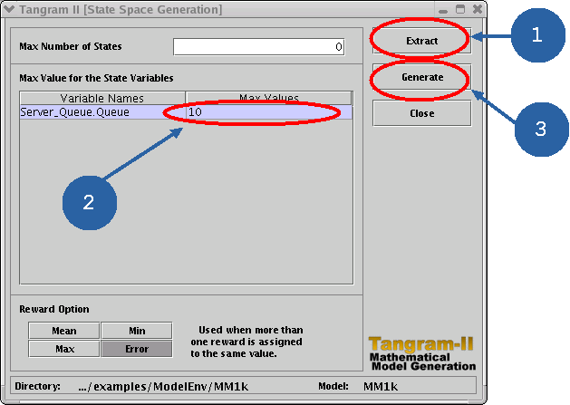
  1.    As soon as you made the desired changes, you can "generate" (compile) the model. In order to do so, first click on the "Mathematical Model Generation" button (marked with a red circle in the screenshot below). Please, refer to the following figures and instructions in order to see how to proceed.


    mev2c
statesp


Click first on the "Extract" button.  Then fill the field that corresponds to the maximum value of the state variable "Server_Queue.Queue" with the value "10" (type 10 and <enter>) and finally click on "Generate".  Note that you may let "Max Number of States" equal to 0 (zero), as default.

excl

Pay attention! Always remember to click on the "Extract" button when you make any change in the tgif model.

The changes will just take effect if you click on the "Extract" button.

Also don't forget to press <enter> after filling in the "maximum values" field.

Just after that click on "Generate".
excl


If, when you type the digits (numbers) in the text box, nothing appears on the screen, do the following. 

First, verify if you are with the focus on the box. 

Then, disable  "NumLock".


note 

Letting "Max Number of States" equal to zero means that there is no a priori bound on the number of states in the model.

note 
The state variable "Server_Queue.Queue" is automatically extracted from the model description.

 In our particular model, we just have one state variable - the size of the queue, which is part of the server object.

Note that the state variable name is composed by two parts: before the dot we have the name of the object which defines the state variable, and after the dot the name of the state variable as specified in the "Declaration" section of the object description.


At this moment, if you take a look at the terminal where you opened the tangram2, you will see something like this:


make -f /usr/local/Tangram2/lib/Makefile.mark_find TANGRAM2_HOME=/usr/local/Tangram2 BASE=MM1k
g++ -O2 -w -g -I. -I/home/daniel/include -I/usr/local/Tangram2/include  -c MM1k.user_code.c
...Finished
./mark_find -G -m 0 -f MM1k -d 0 -w 4
...Finished
Total number of states: 11
Total Execution Real Time: 7.045 miliseconds
...Finished
...Finished
...Finished


Note that our model has 11 states (one corresponding to the empty system, and the other ten corresponding to the system with one, two, ..., ten clients in the server queue).  If, during the "generation" (compilation) of the model, some error occurred (for instance, a syntax error), the error would be reported in this terminal, so that you were able to correct it.  You would need to go to step 9 again.

As soon as the model was correctly compiled, you may now click on "Close".

  1.  Ok. Now the model is generated, so we may solve it analytically or via simulation!  Click on the button marked with a red circle in the screenshot below to solve it analytically!

Note: By "generated" we mean that a Markov chain was generated. The transition rate matrix Q was generated. And we may always obtain the matrix P using the so called method of uniformization! If you want to see the matrix Q, take a look at the file MM1k.generator_mtx.
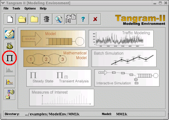
modelenv2e
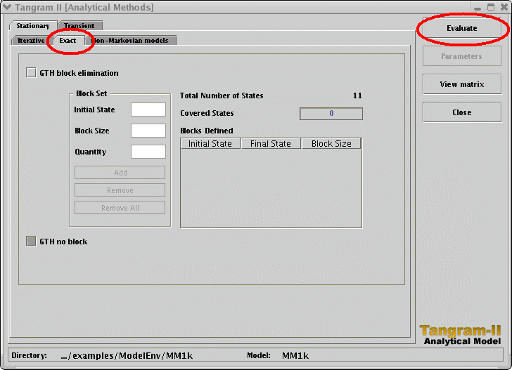
  1.  Tangram-II has lots of solution methods.  We will use the simplest one: GTH (similar to Gaussian Elimination).  Just click on the "Exact" tab, and then in "Evaluate" button, as shown below.  If you want to see the structure of the probability matrix (matrix P of the markov chain) click on "View Matrix".

    solution

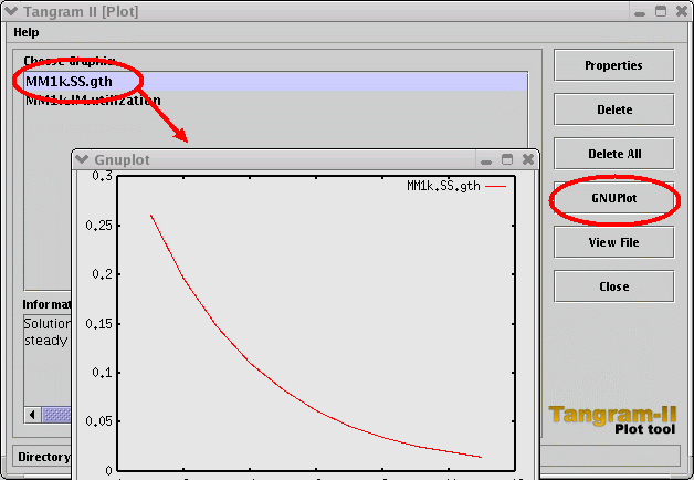
  1.  At this point, the model has been solved ( a system of the type π = π P was solved ) and we have the stationary solution of the system ( the vector π ).  The file which contains this solutions is automatically generated, and is called MM1k.SS.gth (because it's the Stationary Solution of the MM1k model using the GTH  method).

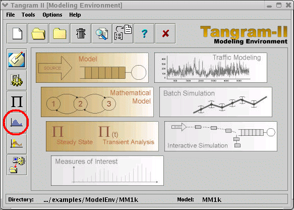
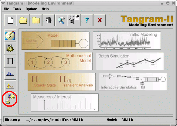
  2. Ok. We may now get some measures of interest.  Suppose, for instance, we want to know the system utilization.  First, we have to open the "Measures of Interest" screen.
modelenvg

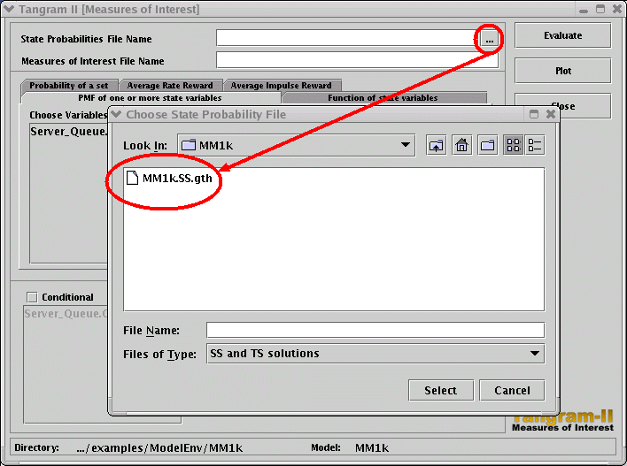
  1.  Let's calculate the server utilization.  That is: the probability of having 1 or more clients in the server.  In order to do so, we will use the vector π which we have just obtained.  Take a look at the image below to see how to do that:

    im1b
    note 

    Note that the state variable "Server_Queue.Queue" was  declared in the model (take a look at the declaration section of the Server_Queue object).  This state variable stores the number of packets in the server queue.


    note 

    You may take a look at the file MM1k.SS.gth, using your preferred text editor, in order to see the steady state probabilities of the states of your model.  In the first column of the file, you have the state number, and in the second one, its steady state probability.


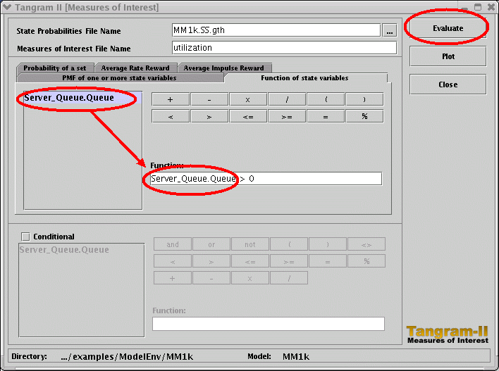
  1. Now, we specify the name of the measure of interest which we want to calculate, and it's formula.  Note that if you click on "Server_Queue.Queue" the state variable will automatically appear in the box of the formula.  Complete it, and then we click on "Evaluate".

    im2b

note 

You may evaluate any function of the state variables, involving  the operators shown on the screen (+, -, / and so on).

For instance, if you would like to evaluate the probability of having the server queue with an odd number of packets, you should use the formula  ( Server_Queue.Queue % 2 ) = 1.


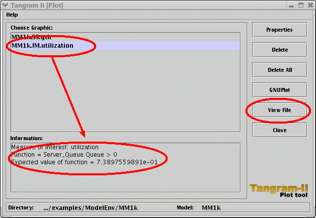
  1.   Now, we would like to see the result!  Click on the "Plot" button.  You will get the following screen.


    img3b

    So, we've got it!  The server utilization is 0.7389 (verify it, solving the M/M/1/k model using pencil and eraser!).

  1.      We may also see the PMF (probabililty mass function) of the number of clients in the queue.  Observe below:

img4b

note 

In our particular model, we just have one state variable. 

If we had more than one state variable, we would need to specify if we want joint distributions or marginal distributions.  In order to obtain joint or marginal PMFs, select the tab "PMF of one ore more state variables" in the screen shown in step 17. Then, select one state variable in the left box, and click on the "Add"  button.  You may repeat this operation if you want joint distributions. Then, click on "Evaluate".


  1.  Ok, so last, but not least, let's simulate the model!

    meg


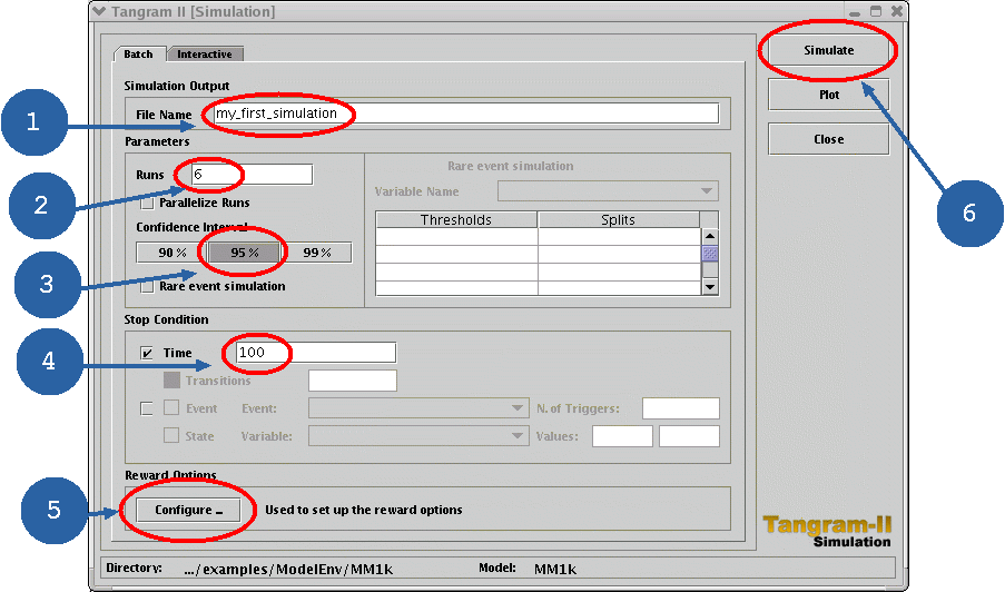
  1.  Let's do a batch simulation.  First, you need to set the parameters.


    simul1b
   The file name (1) is the name of the output file which will store simulation results.  Runs (2) is the number of simulation runs. Each simulation run will take the simulation time specified in the time field (4).  The results will be generated with the confidence interval (3) specified.  The larger the confidence interval, the greater the probability of having the results within that given interval.
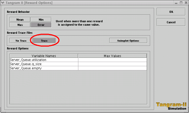
  1. In the configure screen, click on "Trace".  This indicates to Tangram-II to generate trace files of the values of the rewards during the  simulation.


    simul2b

  1.   That's it!  After you click on the "Simulate" button, wait a bit.  The simulation results will be available via some files which will be generated during the process.  For instance, to know the utilization,  you may see the file  MM1k.SIMUL.my_first_simulation.  In this file, using your preferred text editor, look for the following lines:
---------------------------------------------------------------
                 R E W A R D S   R E S U L T S
---------------------------------------------------------------

 Simulation time : 100.000000
 Number of runs  : 6
 Total simulation time : 600.000000
 Confidence interval   : 95%
 Simulation execution real time : 2751.332 milliseconds

----------------- Rate Rewards Results -----------------

 Measure: Server_Queue.utilization
   - CR(t) : - mean = 7.3226132520e+01
             - var  = 3.9265764744e+00
             - interval = ± 1.58557751e+00
               [7.16405550e+01 , 7.48117100e+01]
   - ACR(t): - mean = 7.3226132520e-01
             - var  = 3.9265764744e-04
             - interval = ± 1.58557751e-02
               [7.16405550e-01 , 7.48117100e-01]


    And compare the value of the utilization obtained via simulation with the one obtained analytically!  They agree!

    You may also want to see the file MM1k.Server_Queue.q_size.IR.trace.  This file shows a trace of the evolution of the queue size during the simulation.  Using this file, you are able to know exactly what happened during the simulation (when did each of the services occurred, and when did each of the arrivals occurred).  Then,  using awk or perl (or any other text processor) you can obtain other measures from the simulation, processing the resulted files.

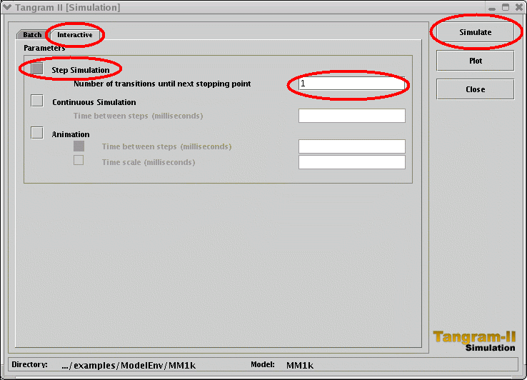
  1.   Finally, you may want to do an interactive simulation, to see interactively how the model behaves as the time passes, step by step.
is1b

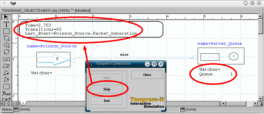
  1. After you click on "Simulate" and then on "Start", you may click in the button "Step" repeatedly, and see how the model evolves as a function of time!
is2b

  1.   We hope you have enjoyed this tour!  Now, start reading the manual!


For further information refer to Tangram2 manual (included with the software) http://www.land.ufrj.br
If you have doubts, which persist even after reading the manual, contact:
support@land.ufrj.br